
A compensated graphic equalizer design approach

This part 2 of the sequence has been rewritten in places to make the operation of the compensation scheme clearer than an earlier version. The graphs have been recreated just to make sure that the process was not lost in the mists of time (the first version was created in 2009 from basic ideas I had in the 1990s).
First of all, in summary:
· All the elements required to create a very high performance stereo ten-band graphic equalizer based on the cascaded bump/dip method are developed and demonstrated in simulation.
· Band center frequencies are chosen, and pre-warped to compensate for the digital implementation.
· The bilinear s-to-z transform (with pre-warping) is used to get standard IIR z-plane biquad coefficients from the bump/dip s-plane transfer function.
· Filter engine coefficient memory values are calculated, turned back into filter parameters, and used in a SPICE simulation model to show the frequency response of the cascaded filter.
· A standard minimum-storage cascadable Direct Form IIR biquad section for the filter engine implementation is proposed.
· The method used to derive the core bump/dip parameters from the desired filter center frequency gain is introduced, and the rationale explained.
· The compensation scheme which allows accurate fitting of the achieved frequency response to the desired band gain values is explained, implemented in Excel, and demonstrated.
· A worked example of an extreme frequency response is given, showing the convergence of the compensation method with only two passes through the algorithm.
· Various secondary issues pertinent to successful implementation and optimal performance are discussed.
Type of equalizer, number of bands, band center frequencies
This report documents a ten-band graphic equalizer based on the cascaded bump/dip approach. It’s trivial to change the number of bands as all the design tools developed for this scheme are scalable. Initial calculations indicate that a stereo ten-band equalizer is at the upper limit of the digital filter engine in the initial target device both for available compute cycles and for available memory.
A suitable starting point for band centers is to use octave band spacing starting at 31.25 Hz (just about the lowest musical note unless you’re a fan of extreme organ music) and ending at 16 kHz (few people can hear reliably at this frequency and there’s certainly no valuable information in any conventional program material at this frequency).
Digital implementation requires frequency warping
This equalizer is to be implemented in the digital domain. The filter parameters will change when the sample rate is changed. This shouldn’t be a problem in a practical system even if successive selections are played at different sample rates (the system might also implement sample rate conversion to simplify this). The function that calculates the filter parameters from the desired gain settings can also take a sample rate selection argument.
To deliver filters centered at the desired analogue frequencies, the actual ‘digital frequencies’ implemented need to be shifted to match the ‘warping’ of the frequency axis which follows from the use of the bilinear transform to implement the digital filters. The frequencies fb for which the filter sections have to be designed in order to get the desired analog frequencies are shown in table 1 for both 44.1 ksps and 48 ksps sample rates; the warping of the frequency axis is clearly significant for the highest frequency filters.
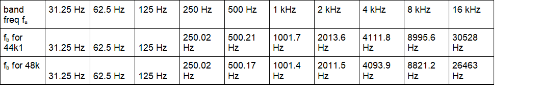
table 1: digital band frequencies fb needed to get analog band frequencies fa
Development of filter response parameters
A standard s-to-z bilinear transform, implemented in a spreadsheet, was used to turn each analogue bump/dip s-plane transfer function
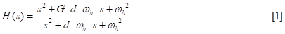
with desired band gain G, required denominator dissipation d (dissipation is 1/Q), and preset band angular frequency ωb=2πfb, into the regular z-plane IIR biquad form:
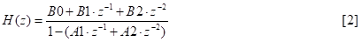
with the denominator structure use of B and A following Lyons [1]. (This is a bit clunky, not the presentation I use these days, but this is an old report).
Some examination of example filter configurations indicated that it made sense here to economize on coefficients by dividing through the numerator by B0 to get
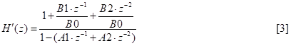
and creating a gain factor to multiply into the overall transfer function at some convenient point:
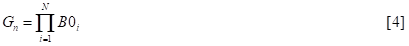
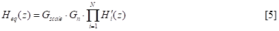
With an additional scaling or centering gain for the whole response (described later) the overall transfer function of the filter is:
Simulation indicates that the typical change in the ‘straight-through’ gain of the filter section far from the band frequency is only moderate when you do this, less than 3 dB for each section.
Calculation of filter engine parameters
The ‘standard’ way of implementing IIR filters on the initially chosen filter engine involves some coefficient scaling in order that all the coefficients fit into the number space used. Coefficients can only be in the range {-1...+1-223}, which is a bit inconvenient since the A1, A2 and normalized B1 and B2 coefficients can lie in the range {-2, +2-222}. So the input signal to a filter section, and the output signal saved in variables for the delayed feedback paths, is left-shifted by a factor of two so it can then be multiplied by a feasible coefficient before accumulating.
In the LTspice analyses for this memo, the implemented coefficient memory values are ‘reversed back’ into a parameter line for a biquad model, so that the consequences of coefficient quantization can be checked. The parameters are fed to an LTspice sub-circuit. The biquad is realized as a continuous time circuit by using a transmission line to model the z-plane time delays:
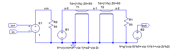
figure 1: LTspice z-plane biquad used for analysis
IIR filter architecture
The basic processing flow for the standard Direct Form IIR biquad block on the chosen engine is shown in figure 2, which is drawn to highlight the requirements for variable storage space. Other processors will likely be similar. As shown, that block requires four specific variables to store delayed versions of the shifted input and output variables (figure 2):
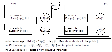
figure 2: basic IIR biquad building block
It’s wasteful of precious filter engine memory if we just cascade these, because the output op(i) and its delayed versions d1op(i) and d2op(i) are also required in the feedforward part of the following section. So after the first section, all we need is to cascade sections of the form of figure 3:
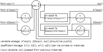
figure 3: cascadable IIR filter block with less storage requirement
Each section has an additional requirement for two more filter state variables (typically held in the data memory) and four more coefficient variables (typically held in the coefficient memory).
Relationship of filter parameters to desired gain
We’ve now developed the filter parameters so that the entire equalizer can be both implemented and simulated. However, we skipped over an important calculation. In equation [1] the parameter G is the ‘slider setting’, the gain that’s required at the band frequency fb. But what is the dissipation value d and where does it come from?
One simple approach is to set the dissipation value d so that it’s just unity in the case of a bump (G>1), or equal to 1/G in the case of a dip (G<1). In the case of a dip, the numerator dissipation becomes unity for all gains. This means that the dip response for gain 1/G is the exact inverse of the bump response for gain G. Two sections, one bump and one dip, designed like this would exactly cancel out at all frequencies.
With the gain varied from -12 dB to +12 dB, this approach produces the results in figure 4, for the 1 kHz band.
This produces plausible results, but closer inspection of the nature of the frequency response curves reveals a difficulty which will hold us up shortly when we start looking at a compensation scheme to make the response correction more accurate.
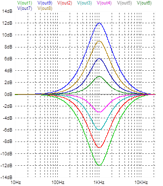
figure 4: 1kHz band curves from -12 dB to +12 dB with simple ‘d=1’ setting
So, without proof here, we’ll introduce first the desired result for calculating the dissipation as a function of band gain:
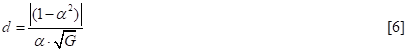
where α is the ratio between the (digital) band frequencies of adjacent filters, in this case approximately 2 (it would be exactly 2 but we’re going to use pre-warped frequencies that ‘stretch out’ as you go to higher values). This produces a subtly different set of curves, shown in figure 5. What makes these curves ‘better’ than those in figure 4?
To see this, look back at the figure 4 curve responses at frequencies of 500 Hz and 2 kHz, for the +12 dB and +3 dB examples. In figure 4 we can see that the gain of the +12 dB curve at 0.5x and 2x the center frequency is clearly more than half of 12, i.e. 6 dB. On the other hand, the gain of the +3 dB curve is visibly less than 1.5 dB at the 0.5x and 2x center frequency points. This illustrates that using the simple constant-Q approach, the response at other frequencies isn’t a simple linear function of the gain response at the band center. A linear relationship will come in very handy and we’ll soon see why. So look now at the same curves in figure 5:
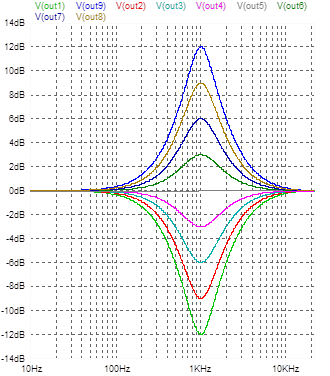
figure 5: 1kHz band curves from -12 dB to +12 dB with equation [6] for d setting
Now we see that the response at 0.5x and 2x the band frequency is exactly equal to half the response in dB at the band center, for both bump and dip, for all gains. This is the constraint that generates equation [6], after some algebraic manipulation of the transfer function. The factor doesn’t have to be one-half, but that special case makes the overall algebra cleaner.
So equation [6] is used in the design to set the denominator dissipation, given the required band gain setting. The numerator dissipation is always the denominator dissipation times the band gain.
An iterative compensation scheme
It’s tempting to ask whether the strict proportional relationship between gains at different frequency offsets in our filter sections applies for all frequencies, after we’ve set it at x2 and x0.5 through equation [6]. Well, it would be too good to be true; it’s only exact at the frequency points defined by that parameter alpha. But the errors at the other band centers are in fact quite small. They are low enough that even for quite wild frequency responses, we can very quickly iterate on a bunch of settings for the ‘actual’ slider values which will give us the desired frequency response.
If the approximation is true that the gain of filter Fi at some band frequency bj is a known constant aj-i times the set gain Gi of filter Fi, then we can write a whole set of equations relating the band settings Gi to the actual overall gain Ej at the frequency bj. Note that both Gi and Ej are expressed in dBs, not linear factors.
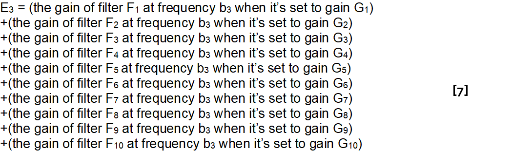
In words, to use band 3 as an example, the gain of the overall equalizer at frequency b3, in other words E3, expressed in dB, is:
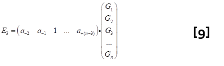
With the assumption of gain proportionality, we can therefore write the equation:

Or in vector format (n=10 remember):
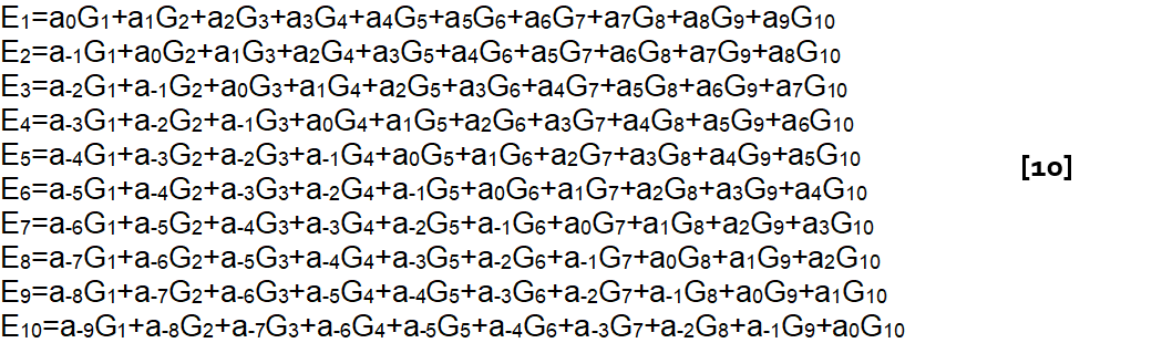
Now if the core filter has a center gain of 1, then a0=1 and our constraint equation [6] forces a-1=a1=0.5. The rest of the ai (note that a-i ≈ ai, they’d only be exactly equal if the frequency ratios were exactly constant, which they can’t be due to the pre-warping) can be pre-calculated as constants, or adapted during iteration, as we’ll see.
We can write down equations for E1 through E10 and hey, presto: we have a collection of simultaneous equations with constant (at each iteration) coefficients telling us what you get (the Ejs) as a function of what you set (the Gis).
Written as a matrix equation, it looks like this:
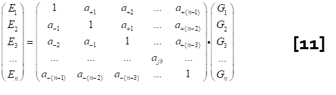
The wonderful thing about simultaneous equations of this type is that they are soluble, in other words, we can easily produce an inverse relationship which tells us what to set given what we want to get.
That sounds like a plan! And it looks like this:
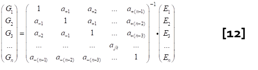
where of course the n Ejs are what we want to see, and the ais are calculated from equation [6] given the Gis that we evaluated on the previous go-round.
Let’s see how this works.
To extract the Gis in the initial test of this approach, the equations were written down in a design spreadsheet and the Excel MINVERSE() function used to develop the inverse solution. For an arbitrarily chosen starting band gain of 0dB (i.e. unity) in every band, the ai look like this (note a little rounding here and there):
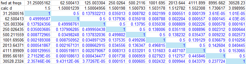
and the Excel-calculated inverse of this matrix looks like this:
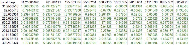
If proportionality were exact for all frequencies, this would be a constant array, and the code would not need to calculate these values at run time. But because matrix 1 is going to depend on the dissipation value (which is a function of the gain setting), the inverse matrix 2 will change as well.
The calculated band gain values (the Gis) are dropped back into the routine which constructs the simultaneous equations, and these cause new dissipation calculations which fine-tune the coefficients in the matrix, causing the solution to be based on assumptions closer to the final value.
Worked example
A standardized ‘whacky’ response was defined, as shown in table 2:
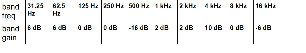
table 2: desired gain response for the example
When these gain values are just set directly as filter gain values (and used in equation 6 to create the dissipation values), you get the overall response shown in figure 6. It’s clearly waving up and down in sympathy with our requirements (X marks the spot where the band slider is set to) but is a rather shabby approximation (though no worse than anyone else’s uncompensated graphic equalizer approach).
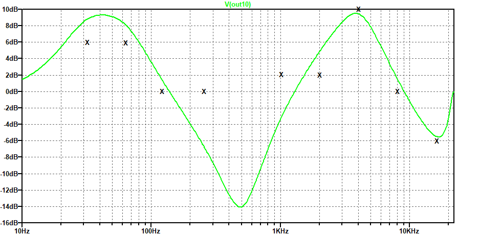
figure 6: just setting the table 2 gain values on the filter sections
We can run the compensating algorithm once, with a starting set of coefficient values ai. What to use? Well, I reckon the closest guess we can make is the gain values we’ll eventually want to implement (to be honest it does not make a lot of difference, you could hard code it as all 0 dB and the end result would not be noticeably different after iteration).
The resultant response is shown in figure 7. Numerically it is closer, though there is clearly some exuberant oscillation of the response, as adjacent filters fight against each other for control of the system gain. The ‘X’ are not quite hit in places.
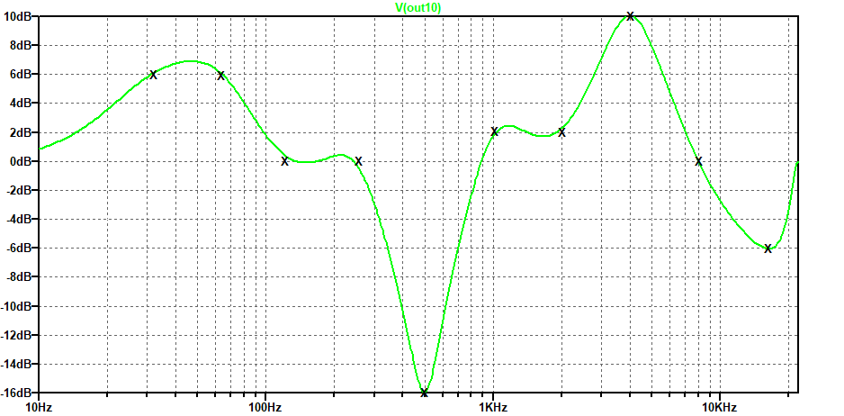
figure 7: response after running the compensation algorithm once
Now we take the gain setting values produced by the first application of equation 12 and use them to create a new matrix and a new gain setting solution. This is much better, in fact, it’s as good as we could hope for, shown in figure 8. Of course, who is to say whether this overall response is suitable for the use to which the equalizer is put. But what you can say is that if the response has to fit a set of frequency points, this method enables you to get there quickly.
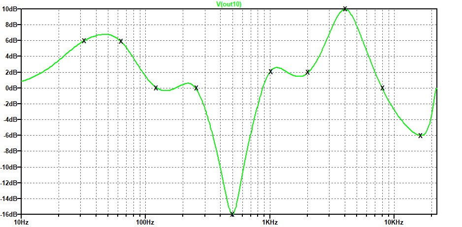
figure 8: response after running the compensation algorithm twice
What do the filter gains look like? Table 3 shows the actual gains required in the filter sections to achieve these results. It would take a great deal of tweaking and cursing to alight upon these values by adjusting one slider at a time and looking at the results on a frequency response analyzer; some of the set values are 12 dB different from the desired band gain settings!
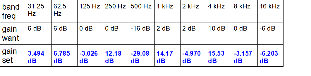
table 3: actual band gain settings for the example
Other issues to take into account
gain centering
If you slide all the gain sliders up by +10 dB, it’s reasonable that you’d expect to get a response which is ‘flat’ and just up at +10 dB. And indeed you do, except it’s not that flat (well, it peaks at +0.4 dB, that’s fantastically flat by normal equalizer standards, but why not aim higher?):
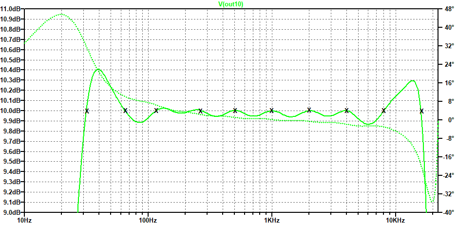
figure 9: optimized response for all bands wanted at +10 dB
The amplitude response in figure 9 is the thick trace, and the thin trace shows the phase response, which deviates a little at the extremes of the audio frequency range. The compensation algorithm was used twice, as in the previous case.
The actual band gains needed to get that response are shown in table 4; note that they look very different from what you’d naively expect:
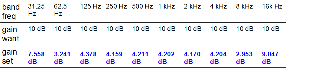
table 4: actual band gain settings to get all at 10 dB
But the question is, why bother? Why not just set an overall channel gain of 10 dB, and leave all the band gains set to 0 dB? This is the degenerate position in which all the responses cancel out, and there’s no ripple in either the amplitude or the phase response. This would clearly be a ‘cleaner’ signal path.
Extending this to a more general case, we can see that adding or subtracting a fixed gain to the overall response could make the fit look nicer and possible sound better. To ensure better performance on these pathological cases, the firmware could just subtract the mean dB gain, and implement a response that’s then balanced around 0 dB. This gain is Gscale, included in equation 5 earlier.
The full design package includes the ability to change the ‘base gain’ to optimize the overall result.
overload and section ordering
This is a perennial problem in cascade filter synthesis. If the filter sections are not ordered optimally, internal overloads can limit the dynamic range. The simplest approach to preventing internal overload is to put the ‘dip’ sections first, followed by the ‘boost’ sections. This ensures that for any frequencies where the output is expected to overload before the input, the output node will in fact be the first to overload.
This is a bit of a pain when someone is twirling the gain of a band up and down through 0 dB. If the band is set to be a dip, the filter section should be towards the front of the cascade. When set to ‘boost’ it should be towards the end. But re-ordering the bands is definitely not something that can be done without a filter ‘stall’ and a brief audio mute to allow the signal to set up again.
The worked example also shows that the combination of bumps and dips can be non-obvious, with sometimes a bump where you’d expect a dip given the gain requirement, and vice versa.
More sophisticated techniques, involving the distribution of gain across filter sections, can yield a slightly higher dynamic range, but are probably overkill at our ambition level here. In terms of dynamic range, though, you might be tempted to ask: “surely with a 24-bit filter engine we have more than enough dynamic range for every eventuality?” In fact, if we allow a reasonable safety margin, we do have to be careful. The boosting filter sections will magnify the truncation noise which is inherent in the IIR filter section, and sufficient overall signal level margin has to be retained to allow for maximum boost plus additional gain margin and transient effects. With 24-bit arithmetic, it should be possible to get overall system numerical noise below a notional 16-bit noise floor, but it will not be massively below. More precision is certainly a benefit here; plug-ins will almost certainly use double precision floating point.
possibilities for section optimization
The numerator and denominator of H(z) don’t interact, and it’s possible to ‘perm’ these separately. It’s possible that improved dynamic range can be achieved by different ordering of numerator and denominator functions, but that’s far too exotic to attend to at this stage. It would also require the deployment of a more generalized IIR biquad section. An optimized approach to the required biquad will be covered in the next part of this sequence.
missing filter sections
Any filter section requiring a gain of 0 dB can formally be removed as it does nothing. Since it is always possible to scale the system gain such that at least one set gain is zero, this does mean that the maximum number of filters needed to make a ten-band equalizer is nine, if this approach is used to set Gscale. Of course, this approach does not guarantee to deliver the best available dynamic range from a finite-precision filter engine.
dynamic updating
Listening to the audio output while twiddling the settings will be deemed essential by most customers. We may have to wrap a little gentle audio concealment around the system to make this feasible, since the individual variables containing filter coefficients are not accessible to system writes when the particular filter engine targeted for the original report is running.
references
[1] Lyons, “Understanding Digital Signal Processing”, 2nd edition