
A partial review of graphic equalizer design approaches

A long time ago I had the task of implementing a decent, high quality audio graphic equalizer on a modest embedded processor as part of our ‘Made for iPod’ program. We implemented the control as an iPhone app - subsequent articles will show some pictures. The technique that will be described in those articles is absolutely ideal for the modern plug-in approach. This is a light edit of a report I kicked the project off with.
This article provides a brief overview of the nature and variety of audio equalizers. Then, it gives a broad outline of various audio equalizer design methods. As well as classical analog approaches, it describes digital methods that suit fixed-point digital filtering engines. An attractive candidate is an implementation of multiple bump/dip IIR filters in series.
Subsequent reports will document the structures and calculations and present example responses for a complete 10-band audio equalizer (31.25 Hz to 16 kHz bands in octave steps). This will be implemented as a series cascade of IIR bump/dip sections. Channel dissipation (that’s the reciprocal of Q) values will be dynamically calculated from the required gain/dip values at band centers. A response compensation method guarantees the fit of the equalizer’s frequency response to the called-for band center gain values.
What is an ‘equalizer’, in this context?
Equalization is a rather generic technical term. This report covers a specific class of audio equipment referred to by the unmarked term ‘equalizer’ or by marked terms such as ‘graphic equalizer’ or ‘parametric equalizer’. It doesn’t cover the equalizing circuits used to correct the replay response of phono cartridges or tape heads. It also doesn’t cover the cable loss compensating equalizers used to extend the transmission length of cables handling high-rate audio/video data such as HDMI.
An equalizer, then, is a circuit or product capable of altering the spectral balance of an audio signal. In-system, an equalizer is in principle capable of ‘equalizing’, or flattening, the replay frequency response of an audio reproduction chain. In practice, many equalizers are deployed not to improve accuracy but to emphasize elements of a sound mix for greater audio ‘impact’. They are essentially complicated tone controls in that context.
In the all-analog days, equalizers were broadly classified into the groups ‘graphic’ and ‘parametric’. Graphic equalizers enabled the creation of a coarsely-described frequency response by means of sliders or peg-in-socket boards, whose appearance mimicked a frequency response, generally on a logarithmic (dB) scale. The more ‘technical’ parametric equalizers gave extra control over the response-shaping filters, typically specified by parameters such as center frequency, height/depth and bandwidth. These filter sections can be individually and iteratively directed at system frequency response defects by an experienced sound engineer.
In the digital era, the graphic-parametric implementation-level distinction has become somewhat blurred; the modern approach is to create a user interface showing the implemented frequency response and give the user various methods for interacting with this in order to yield the desired changes. The underlying architecture could be similar in either graphic or parametric forms, or indeed be implemented using schemes that have no practical analog equivalent.
The age-old tone control (I know it as a Baxandall tone control after the English audio expert who is credited with first proposing it) has just two frequency bands of control; you could think of it as a two-band graphic equalizer. In the 70s, amplifiers often acquired an additional ‘middle’ control, while electric guitarists will be familiar with the ‘presence’ control, capable of boosting those frequencies near the peak sensitivity frequency of human hearing, with a notable advance (if that is the correct term) in loudness and stridency.
Many cheap home-audio-in-a-box systems these days have at least a five-band equalizer (low and high bass, midrange, low and high treble). Various listening ‘presets’ are sometimes supplied, ostensibly suited to classical, pop, jazz, rock and other types of source material.
An equalizer for the home or semi-professional musician is likely to have around ten bands of adjustment; at this level, a filter section for every octave of the musically relevant audible range is available. This allows reasonable control of voicing interactions in a multi-instrumental mix. In a pro recording environment or traditional sound reinforcement system, it is not unusual to see third-octave systems with around 30 filter bands covering the audio band. However, sound reinforcement systems are moving to more sophisticated forms of time domain audio processing, which analyze venue acoustic defects with a calibration microphone. A dedicated combination of FIR digital filters and feedback-tracking notch filters then polices the signal, evening out interference effects and enabling significantly higher sound levels. As if the iPod generation needed any more help in developing premature deafness...
For embedded designs (and simple plug-ins), graphic equalizers with fixed band centers and between 5~10 bands will be the most likely. The equalizer design method that will be proposed later is flexible, and the band count will be limited only by the number of filters which can be implemented in real time in the chosen filtering engine.
Methods of equalizer implementation
This report doesn’t consider methods (either filtering or FFT-type) in which the entire frequency response is implemented “in one go” by mapping a complete transfer function to the entire response and implementing that. Some advances are being made in that space, but it is usually deployed for the correction of the frequency response deficiencies in a product such as a speaker, rather than for the run-time user-driven manipulation of the frequency response.
sum of parallel bandpass filters
This method is simple to implement either in the analog or digital domains. It’s the basis of the Microchip equalizer library whose description (it’s an old-style link and your browser may object) can be found at
http://ww1.microchip.com/downloads/en/DeviceDoc/70347A.pdf
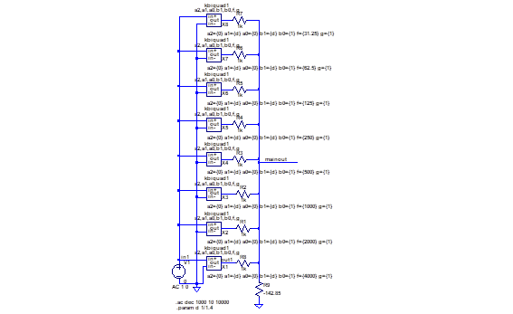
figure 1: simulation approach for sum-of-bandpass equalizer (analog)
The outputs of a bank of bandpass filters, all fed from the input signal, are added together. Gain weighting coefficients are used which correspond to the notional ‘slider’ settings of the equalizer. In this implementation, all these coefficients are positive, that is, each channel has a selectable linear gain between minimum (often zero) and maximum values.
A significant disadvantage for ‘quality’ audio applications is that the equalizer affects the phase shift through the channel even when all the band gains are set the same to yield a gain-frequency response that’s as flat as possible. This unnecessary effect on the phase shift is generally deprecated in the audio world.
The Microchip documentation implies eight octave filter bands with a Q of 1.4. This leads to a very poor amplitude and phase flatness (ignore the static gain offset, which is not compensated in this plot). The accompanying graph uses the band frequencies defined in the Microchip documentation; it’s not intended for operation across the full audio band.
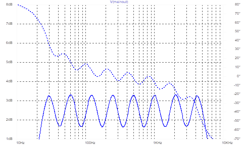
figure 2: predicted Microchip library response, ‘flat’
What I think they meant to say is that the dissipation (=1/Q) of each section should be 1.4; this gives a very much flatter amplitude response, and a phase response which is much more linear – although only as a function of log(frequency), which is not very useful.
This approach is not really suitable for use in any quality audio product, even at the low end. Therefore, no further worked examples will be done using this technique.
If the bandpass filters could be implemented as linear phase filters with matching delay, the phase shift issue could be evaded. Efficient structures to implement parallel banks of bandpass filters exist (they are used in some audio compression methods) but they are not completely suited to this purpose because they rely on alias cancellation which is broken if the relative gain through summed filter channels is adjusted.
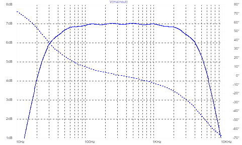
figure 3: what Microchip probably wanted; same scale as figure 1
Note also that this architecture has an inherent bandpass characteristic, because it is the sum of bandpass responses. It has no transmission at very low or very high frequencies. This is not always a problem, but it does mean that the filter bands need to cover the entire frequency band and can’t just be concentrated where the adjustment is needed.
In some designs, the low and high ‘capping’ filters at each ‘end’ are replaced with a lowpass and a highpass filter respectively. Matching these filters to the bandpass filter responses causes further difficulties in design. (To be fair, I don’t know for certain that the Microchip design doesn’t use lowpass and highpass capping filters; there are no frequency response plots of the implementation, and that always makes me suspicious).
feedback control methods
These are the ‘classical’ methods of audio equalizer design. There are two common configurations following the same general principle. The first technique sums the outputs of the bandpass filter sections to the inverting input of a summing amplifier. Each filter’s input is fed with a mix of input and feedback signal, and the ratio of these signals strongly (but not uniquely) determines the overall gain within the frequency range of that filter.
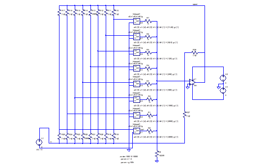
figure 4: a feedback-type analog equalizer, first type
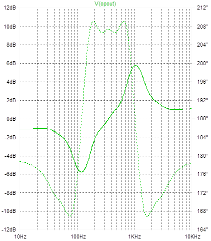
figure 5: a sample eq response from the analog simulation
With a ‘slider’ set positive, the feedback produces a gain of greater than unity – a bump. With a negative setting, the gain is less than unity – a dip. With all ‘sliders’ set to zero dB, the feedback factor has no frequency dependence and the through response of the system has the amplitude and phase response of the main signal path amplifier, which can be made completely benign in the audio range.
The interaction between filter sections limits performance. The ‘sliders’ in figure 5 were set to give -12dB at 125Hz and +12dB at 1kHz, but we only got +/-6dB. Reducing the filter dissipation (unity, in this graph) makes the peaks and dips more accurate, but dramatically disturbs the response ripple.
The second technique is similar, but the filter networks are used to simulate an impedance which is connected so that the split between signals sent to the inverting and non-inverting inputs of an opamp is varied according to frequency. In an analog design this approach has the advantage that grounded impedances can be used, which are easier to implement actively.
The feedback approach causes significant difficulty when a digital implementation is needed. This is because the inherent delay through a digital filter affects the frequency response of an IIR equalizer in which (digital) feedback is wrapped around the filter sections.
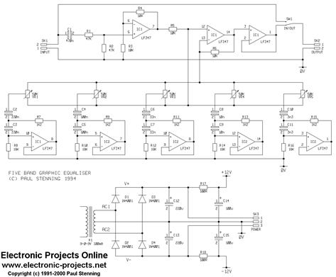
figure 6: a hobby-grade example of type 2 analog feedback equalizer
feedforward sidechain bandpass methods
This approach is a combination of the previous methods and is more suited to digital implementation. The main signal goes ‘straight through’, and the outputs of bandpass filters fed from the input signal are added or subtracted from the signal path. Adding a bandpass signal causes a bump, while subtracting one causes a dip. The dissipation factors of the bandpass filters are normally set to give symmetrical bump and dip responses, as this is what users usually expect.
Conventional equalizers have some interaction between frequency bands. With this method, as with the previous one, the interactions are difficult to compensate because they are not ‘linear’. By this we mean that the response error caused by two slider settings together is not the sum of the errors caused by each setting individually (whether this is measured in linear or dB terms). The cumbersome complex arithmetic needed to predict the frequency response is a poor fit for a low-cost micro.
A rearrangement of this approach yields a solution to this problem, as the following section shows.
cascade of bump/dip filters
This equalizer is a cascade of bump (rising at the center frequency) and dip (dropping at the center frequency) sections. The individual sections all contribute to the overall frequency response but they do not interact in the same complex way that the filters in the parallel implementations do. In effect, this approach is the series cascade of a number of single-slider feedforward sidechain equalizers.
In the analog domain, this approach is a difficult choice because the series connection of filter sections encourages the build-up of noise in the channel. In the digital domain, with sufficient filter implementation precision, the noise problem can be made insignificant. In particular, it’s an ideal methodology for a workstation plug-in.
These bump/dip filters can be implemented in several ways. The simplest one is to directly implement the second-order function representing the bump or dip using a standard IIR section, which is a good fit on most filtering engines.
To get the best out of an IIR bump/dip filter architecture, we will need to be careful with the ordering of the filter sections. Each of these sections generates its own noise (through the truncation of the accumulator output prior to internal feedback) and, if it has a peaking character, can also boost the noise generated by previous filter sections. The most defensive strategy involves placing the sections implementing dips first, in increasing order of dip depth, followed by all the peaking sections in increasing order of peak height. This ensures that if clipping occurs, it occurs first at the output (where it can be detected) and not at some unmonitored internal node.
The amplitude response of the channel in dB is just the sum of the dB responses of all the individual sections, which is not the case for the parallel versions previously discussed, where interactions between bands cause the response to vary in a way that is difficult to allow for. This means that the user needs to keep adjusting multiple bands, often significantly, to drive the frequency response to where they need it to be.
Because the frequency response of this circuit approach is a simple linear function of the settings (in dB) of the sliders, a straightforward mathematical approach has been developed which dramatically improves the ‘fit’ between the slider settings and the frequency response. A set of linear equations links the dB response at each slider frequency to the slider settings. It’s tempting to ask whether these linear equations can be solved exactly, to obtain a new set of ‘slider values’ for the filter bands which, when implemented, delivers the demanded frequency response.
With the addition of a constraint relating the individual selected filter band gain and the dissipation factors of the numerator and denominator polynomials, it turns out that there is indeed a closed calculation for a very good approximation to the ‘correct’ filter parameters. And furthermore, the errors are small enough that, almost always, a single iteration and recalculation will reduce the errors to audible insignificance. A great advantage of digital filter sections is that all the bandpass filter parameters can be continually adjusted for optimum performance in a way that analog circuits cannot realistically be.
This approach will be developed in the next articles in this sequence.