
An Excelent fit, Sir!
No, not a spelling error.

This was my first foray into using Excel to bend transfer functions and circuits to fit requirements. You’ll see a lot more of this in pieces to come soon. An apology for some of the equations; in the time since the first writing, Microsoft obsoleted a perfectly good way of creating equations so I had to use the ‘new way’ for some updates and additions to fix some initial omissions and comments. And more apologies for the variable image width - note to Substack folks: please make this more adjustable…
This is the first of two pieces showing a simple technique for designing, optimizing and calculating coefficients (in the continuous domain, suitable for an analog implementation) for a frequency-response-equalizing filter for a sensor. The second part will look at a method for converting it to a digital form for implementation in an MCU or FPGA.
Figure 1 is the first piece of our story. It’s the curve of the sensitivity of a customer’s sensor versus frequency (what kind of sensor, do you think?):
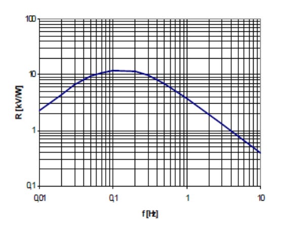
Figure 1: frequency response of the sensor used.
The customer said they wanted to equalize this so that the final sensitivity would be “independent of frequency”. Now, an elementary rule of Filter Wizardry is: the frequency response of a filter doesn’t stop at the edges of the graph. It’s important to understand what the response should do outside this range. “Don’t Care” doesn’t mean “Don’t Need To Care”.
Now, I’ll wager that the response of that sensor continues to fall off at 20 dB/decade outside the graph limits. But it would be a terrible idea to boost the response with gain that continues to rise without limits. We’ll want the response to flatten off or even fall back down, to avoid noise problems. For a first try, let’s hold constant the desired response outside figure 1’s frequency range, for one extra decade in each direction; figure 2:
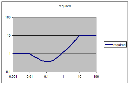
Figure 2: extend the response a decade on either side.
Next, we’ll try to design a realizable filter with a frequency response approximating this curve to an acceptable error. The low frequencies involved indicate using a digital filter to avoid bulky external passive components. The digital stuff is for the follow-up piece; first, let’s design it in the analogue domain.
Figure 2’s response is flat at one end, wavy in the middle and flat at the other end (with apologies to Monty Python); that’s a second order ‘shelf’ equalizer. The amplitude response of the general second order transfer function or ‘biquad’ section:

is easily computed in a spreadsheet. With ω equal to the input frequency divided by the frequency to which the transfer function is normalized, a bit of manipulation gives:

Figure 3 is a clippet of a working spreadsheet, using one column for each biquad section, with the cell formula shown in glorious ‘Excelcolor’. The gains of all the sections used are multiplied up (linear gains, not dB) and deposited in column G:
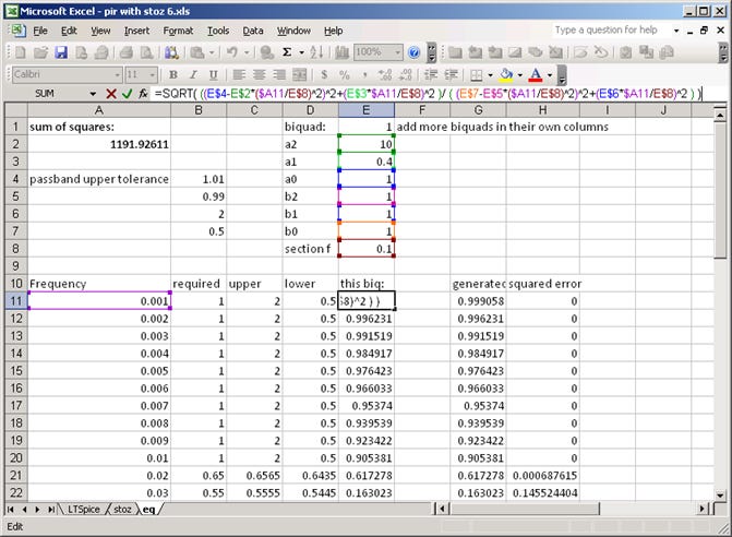
Figure 3: working out the filter response in Excel.
Now we need an initial coefficient guess; here’s how I’d do it:
1 the middle of the frequency range is around 0.3 Hz so that’s where we’ll normalize everything to.
2 at high frequencies we need a gain of 10, so that’s the ratio of the s2 terms.
3 at low frequencies we need a gain of 1, so that’s the ratio of the constant terms.
4 we need a guess at the dissipation, which is the reciprocal of the ‘Q’ of the denominator, and sets the denominator s1 term. The filter covers a frequency range of about 1000:1. My guess is the square root of this, say 30.
5 at mid frequencies we need a gain of 0.4, and very roughly indeed we can set the ratio of the s1 terms to this. In other words, I’ve guessed:

Check out the response – already not bad, figure 4:
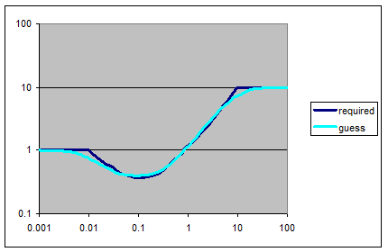
Figure 4: my initial guess.
It’s not perfect; let’s get the spreadsheet to find us a better fit. We need response limits, and a measure for how far out the result is. We’ll use the “method of least squares”. For any point whose gain goes outside set limits, take the square of the relative gain error (1‑generated_gain/required_gain) at each frequency, and add ‘em all up.
For the response limits shown in figure 5, I allowed 1% gain variation in the passband, and between (2x required) and 0.1 in the bands outside. If a response point lies between these limits, it doesn’t contribute to the error function.
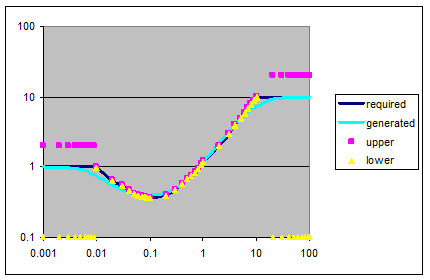
Figure 5: you’ve got to set limits.
Now we use Excel’s Solver to ‘improve’ our response. Configure it to minimize cell A2’s value by adjusting the cells holding the filter coefficients (allowing only positive solutions), and click ‘solve’ to get equation 3a and figure 6:

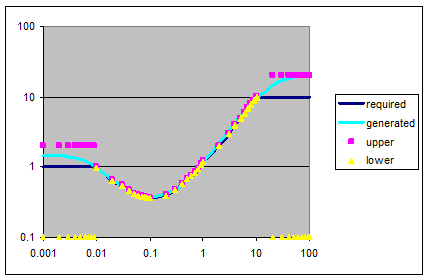
Figure 6: as if by magic, a better fit.
Actually, I’m making it look a little easy. Excel’s solver can be prone to settling on a poor local minimum if your initial guess is too far out, so you sometimes need to intervene to help it (note: more recent Excels seem more stable).
This seems good in the desired frequency range, but that gain is still high outside the passband, especially at the higher frequencies. How about adding another filter section to chop off the low and high frequencies? Separate single pole lowpass and highpass filters would do. But did you realize that you can combine those single pole filters into one two-pole bandpass? It means we can reuse the spreadsheet formula we already created. I’ll try adding a section with the same denominator as my first guess, but with only the s1 term in the numerator non-zero, set to match the denominator:

Let’s also be more aggressive with those upper gain limits, forcing them to fall back outside the band, figure 7:
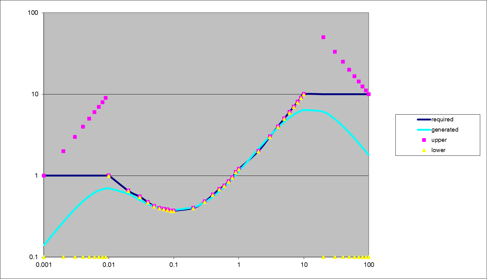
Figure 7: adding a bandpass to reduce the out-of-band stuff - before Solver runs.
We invoke the solver again which gives us equation 5, resulting in figure 8:

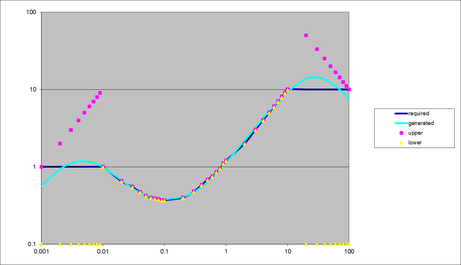
Figure 8: final design with band-limiting, after Solver.
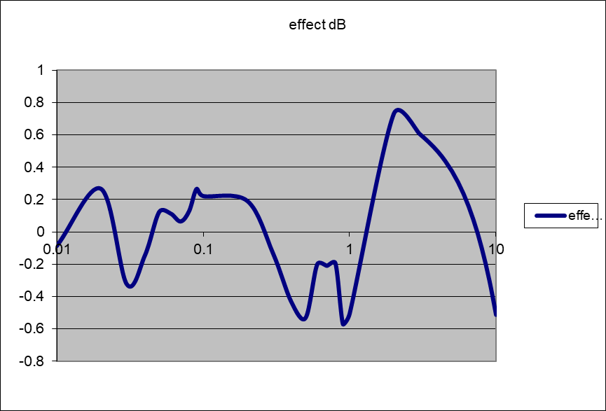
Figure 9; the fit error in dB (the wobbles partly due to my eyeball estimate from figure 1)
which falls away nicely on both sides. It’s still a continuous time design suitable for analog implementation; in the follow-up article we’ll look at issues involved with ‘turning it digital’ – in the same spreadsheet – then implementing it and analyzing it. Let me know if this workflow could be a… fit for you.