Which filters are Noisier – Analog or Digital? Part 2

Seems like people wanted this second part uploaded promptly!

In Part 1, we ran SPICE noise simulations on a simple second-order lowpass filter. We saw that there is something fundamental about the ‘hold’ that the filter’s capacitor network has over the total output noise level. Scaling all the filter’s resistors by a constant factor, to change the cutoff frequency of the filter without changing any of the capacitor values, leaves the total noise voltage unchanged. With practical amplifiers, the noise level is degraded from the ideal case, but it’s still pretty straightforward to predict what they will be.

Can we make useful noise level predictions if our filters are implemented digitally? In modern electronic product design, one can often make a choice between analog and digital signal processing. With analog processing, the filtering and other signal manipulation is done before converting the signal to digital (if it’s indeed ever converted). The digital model involves converting as early as possible in the signal chain, doing the processing in the digital domain, and then perhaps converting back to analog.

So, analog or digital? To help make the choice, systems engineers need a reliable method for directly comparing the noise performance of analog and digital filtering approaches.

We’re taught that “going digital” creates quantization noise, which is the per-sample error involved in fitting a value of arbitrarily high precision into a lower-resolution number system, usually an N-bit binary system with 2^N available states. For any real-world signal, this error is completely uncorrelated with the actual signal and therefore can be treated as random noise, whose value is uniformly distributed between -0.5 LSB and +0.5 LSB. Textbooks demonstrate both that this noise is ‘white’, i.e. has a frequency-independent spectral density, and also that the rms value is {LSB}/sqrt(12), when integrated from DC to Nyquist.

Quantization noise is different from analog noise in one particular way: it’s deterministic. Process an identical signal a second time in your system and you’ll get the same error again. In an analog system, the noise is different every time.

To level the playing field in our comparison between analog and digital filters, let’s assume that input signals are converted to digital, either after the analog filter or before the digital filter, using enough bits of resolution that this input quantization noise can be neglected. I’ll use 20 bits of input resolution in the examples here. Also that our signal processing is done to at least this resolution, if not higher, so that there’s no internal reduction of resolution in the digital case that might affect the results. I’ll use 24-bit integer arithmetic for the sake of example.

With all this, you might be thinking that I’m setting up a false dilemma. Digital filters contain neither noisy opamps nor noisy passive components. So, if we’ve taken the input quantization noise and signal levels into account, aren’t our digital filters going to be essentially perfect and noise-free, running with 24-bit arithmetic on 20-bit data?

It’s a fair question. If the only noise that a digital filter implementation suffered from was the basic quantization noise associated with the resolution of its processing path, we’d have little to worry about. But – and here’s the ‘kicker’ – this isn’t the case, at least, not for the filter topology that you’re most likely to use because it’s the one given in all the textbooks and filter design packages; it simplicity means that software filter designers usually use this too. That topology is the Direct Form filter, the most common form of which is shown in figure 1. We’ll soon see that we do indeed have a noise problem. But first, we need to figure out how to actually analyze the circuit.

Figure 1: the Direct Form I filter that we’ll use here (from Wikipedia).

Like other digital filters, the Direct Form filter is built around unit time delays equal to the sample interval. Such networks are easy to analyze in SPICE because this time delay can be modeled exactly with a transmission line component, which works well in both time domain (.TRAN) and frequency domain (.AC and .NOISE) simulations. It simply delays the signal applied to it by the time specified by its value. It has a flat frequency response and a constant value of both group delay and phase delay.

Figure 2 shows a suitable interconnection of SPICE primitives on an LTspice schematic, with a behavioral source implementing the summing node that creates the desired filter output. At this stage the output voltage is calculated as a floating-point number. But to model an actual implementation, we somehow need to include the effect of (in our case) a 24-bit quantizer. So we need a model of a quantizer that can be used in a linear SPICE analysis. You might think that this is a tall order, because quantization of samples is inherently a non-linear time-domain process.

Figure 2: A Direct Form filter built using SPICE primitives (in LTspice).

Here’s how we do it. If the quantization noise in a digital signal processing circuit can be thought of as a white noise generator as we’ve already suggested, then we should be able to replace it with a different white noise generator with the same rms amplitude and noise spectral density, without affecting the amplitude or spectral properties of the system’s output noise. If this is the case, then let’s replace the quantizer with SPICE’s standard equivalent continuous-time noise source – a resistor! This way, the noise impact of the quantizer can be evaluated in the same noise simulation that’s simultaneously working out the noise of the analog filter in the comparison.

What value should this resistor be? Well, the rms noise voltage contribution of a resistance of value R, measured in a bandwidth Δf, is given by equation 1:

where T is the absolute temperature and k is Boltzmann’s constant. If we define our system full-scale as unity, the rms value of the noise voltage from the quantizer is as shown in equation 2:

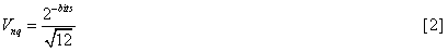
which is the standard result, as mentioned previously. Simply squaring and equating these, we have equation 3:

since Δf is one-half of the sampling frequency. So the quantizer reduces to a resistor whose value is calculated from the sample rate and the number of bits of resolution as shown in equation 4. We put that resistor in series with the signal being quantized, and buffer it with a voltage-controlled source to prevent any interaction with the rest of the circuit. The modified filter circuit is shown in figure 3.

Figure 3: noise simulation schematic for a standard Direct Form biquad.

The SPICE transmission line has a defined impedance, with which it is terminated. To ensure that this impedance doesn’t affect the noise calculations in any way, it is set to 1 micro-ohm in these simulations. The calculated noise-equivalent resistance value of a 24-bit quantizer is around 0.81 ohms for a 44.1 ksps sample rate. The wonderful thing about simulation is that you can deploy quite impractical component values in the service of problem-solving.

OK, we’ve now got all the pieces we need. Figure 4 shows not only the analog filter from part 1 (including the impairments expected from the NE5532 opamp), but also a digital filter (it’s hidden inside a small schematic symbol just to make the schematic more compact). The values for the z-plane transfer function are calculated on the spreadsheet; the cutoff frequency is ‘prewarped’ so that it ends up at the correct value. The Direct Form multiplying factors are trivially related to the transfer function coefficients; all you need to do is invert the sign of the feedback (denominator) coefficients. A 20-bit quantizer is added after the analog filter, and before the digital filter. This quantizer is simply a resistor of the appropriate value, buffered with a controlled source to prevent interaction.

Figure 5 shows the realized frequency responses of the digital filters over the same 10 Hz to 3160 Hz range we used for the analog filters; compare this with figure 2 of part 1. All the digital filters have a response that falls away more rapidly as the frequency approaches Nyquist (one-half of the sampling frequency of 44.1 kHz). That’s a by-product of the bilinear transform approach to filter design (I’ll post some notes on that sometime),

Figure 4: analog and digital filters calculated on the same schematic.

Figure 5: Stepped frequency response of the digital lowpass filter.

What happens when we run a noise analysis? Well, the results are shown for comparison in figures 6 ( analog) and 7 (digital), and the integrated noise values given in table 1. You’ll see that a rather wider scale (logarithmic) is now needed to fit the noise density plot of the digital filter.

Figure 6: Noise spectral density of analog filters.

Figure 7: Noise spectral density of digital filters.

Table 1: Simulated noise of analog and digital filters with same cutoff frequencies.

This data should dispel once and for all the myth that digital filters aren’t noisy. With ‘only’ 24 bits of signal processing, the Direct Form filter is inferior to the analog filter at frequencies below around 300 Hz. At a 10 Hz cutoff frequency, the digital filter’s noise level is worse by 34 dB than the analog filter. It’s ironic that people often cite digital filters as being of most use in replacing low frequency filters that need high-value capacitors. We can see, however, that the active filter comprehensively trounces this particular digital filter at low frequencies. The scaling is definitely not working out as you might have expected!

Where does this noise come from? Well, it originates in the quantizer, but it is hugely magnified by the noise gain of the Direct Form filter, which approaches infinity as the cutoff frequency approaches zero. Whoops. One way of thinking about this is that at low cutoff frequencies, the feedback terms in the filter contribute positive feedback that increases the gain of the filter to the noise terms. The input signal is attenuated by the feedforward terms in order that the through gain of the filter comes out right. The net result is a huge magnification of the noise contributed by the inherent quantizer at the output of the filter calculation.

One way of mitigating this noise is to increase the bit depth of your arithmetic. We could make the 10Hz digital filter match its analog counterpart if we ‘widened’ our system data width from 24 bits to 30 bits. If you’re designing your own chip from scratch, this may be feasible and justifiable, but that’s rare – usually you’re designing with a standard processor (and not necessarily one with processing power to spare, in high channel-count applications).

All is not lost for the digital filter approach, though. For people who need to make decent low-frequency IIR filters using modest processing widths, there are other topologies that don’t suffer the noise gain pathology of the Direct Form filter, and that deliver far superior noise performance for a given processing width. If you’re writing software, the code is going to look rather more complicated, though. The same techniques shown here can be used to simulate the noise performance. That’ll have to be the topic of a future article.

Until then, keep an eye on your use of the Direct Form filter at low cutoff frequencies relative to the sample rate; its noise gain might be your loss. Or just keep it analog!