


Bruton Charisma: Make Those Inductors Vanish Using Savvy Scaling

The title of this piece was, and still is, a combination pun and ‘Pop Quiz’ reference to a 1980 album that’s still a favorite of mine. Can you name it?
I must confess that I just didn’t realize how much mess the monkeys would leave in the Monkey House when I let them loose with a few innocent software tools during the development of “Filter Design Using the Million Monkeys Method”. This piece is the third sequel to that article, and I am still flushing out the little promises that got made in that episode, and in “Match Point: Why Maximum Power means Minimum Sensitivity”.
Most recently, you might have felt as if left hanging by a finger at the end of “Dualling Master: Swap Current and Voltage for Easier Filter Design”. We set out to eliminate the inductors in our LC lowpass filter – and ended up doubling the number of them! We’ll see shortly just how these can be made to disappear in one mathematical stroke.
But first, let’s talk about impedance scaling. In the text that follows, I’ll use ω to indicate angular frequency (2*pi times ‘actual’ frequency). Our filter uses source and load resistances of 1 ohm. Now, if all the impedances in the network change by the same factor, the voltage transfer function – a dimensionless value which is only ever determined by ratios of impedances in a network – is unchanged. So it’s easy to scale the filter to make it suit source and load resistances of, in this example, 1 kilohm. The impedance of an inductor, Z=jωL (I don’t have to explain what j is, I hope) is proportional to its inductance, so we just make all the inductor values 1000 times higher. We also reduce the capacitor values by 1000, because their impedance is inversely proportional to their value, Z=1/(jωC).
The scaled circuit is shown in figure 1, ready for simulation. The cutoff frequency is unchanged from the original 1/(2*pi) Hz; one way of convincing yourself of this is that the product of any inductor and capacitor pair is unchanged by the impedance scaling we just did.
The values are even less practical than they were before. We’ve taken inductor L`3, for instance, from its previous already-enormous 1.621 Henries to a gigantically bizarre 1.621 kH – yes, that’s kilo-Henry, not kilo-Hertz with a missing z. I’ll forgive those inductor-fearing readers for feeling that things are just getting worse and worse! But just hold on for a moment longer.

Figure 1: Same as figure 3b from “Dualling Master”, impedance-scaled by 1000x.
In 1968, Leonard Bruton, working then at the University of Newcastle in the UK, introduced a simple yet beautiful technique to the filter design world. It is sometimes known as the Bruton Transform, though it’s not a functional transform but ‘just’ a scaling. It’s one of the most underrated insights in all practical network theory. He realized that you could scale the impedance of a component by a factor that’s not just a simple real constant, and that interesting things could happen if you chose that factor carefully [reference 1].
Bruton asked: what would happen if I scale the impedance of every element in this network by a factor of 1/(jω). Let’s investigate. If I multiply a resistor R by an impedance scaling factor 1/(jω), I get a new impedance of Z`=R/(jω). But hang on – that’s just the impedance of a capacitor with a value of C`=1/R. By doing this scaling, we’ve made a new impedance that can be realized by a physical capacitor. We’ve “turned the resistor into a capacitor”.
What happens when we scale the inductor? Its new impedance is Z`=jωL/(jω), i.e. Z=L. In other words, it’s a real, frequency-independent constant value L. This can be delivered by a resistor of value R`=L. We’ve “turned the inductor into a resistor”. Isn’t that just the most wonderful thing? There we were, wondering what we were going to do with these six inductors, and at a stroke we just managed to replace them with six resistors. Result!
Just one more thing to do; let’s scale the capacitors in the original network. The new impedance is Z`=1/(jωC) times 1/(jω), and since we all know that j*j = ‑1 (yes?), this can be written as Z`=‑1/(Cω2) and that’s the impedance of an, er, well, what, exactly?
Well, we can see that the impedance is real (there’s no j there), it’s negative, and it depends on frequency. Imaginatively, this new element is sometimes called a Frequency-Dependent Negative Resistor, or FDNR for short. In the golden days of analog filter theory it was also called a “supercapacitor”, but that was before the multi-Farad barrier supercapacitor components used for memory backup and energy storage were introduced. I like the name “D-element”, with a value of D, for which the impedance is Z = -1/(Dω2). So we have “turned the capacitor into a D-element” whose numeric value is the same as the original capacitor’s.
The commonly used symbol for the D-element is like a capacitor but with four (occasionally three) bars instead of two, and easy to draw with the symbol editor in your favorite simulator (and if it isn’t, then why aren’t you using my favorite simulator?). Figure 2 shows our original 1 ohm filter on the left, and the Bruton-Transformed network on the right. No frequency response plot is needed – they are identical.
It’s straightforward to create a suitable D-element subcircuit for simulation from a few controlled sources and impedances, but I’ve not shown it here. Try working out how to do it yourself.

Figure 2: Our original filter, before and after ‘Brutonization’.
Now, before you head to the DigiKey website to order some of these D elements, muttering under your breath that this is another darned class of components to enter into your inventory system, you need to know something. And that is, that the D-element is not a physically realizable, purchasable passive component. It needs a source of energy – can you see why this must be so?
But, although the D-element is not a component as we normally use the term, we can synthesize it nicely using regular electronic components – particularly when one end of it is connected to ground. And (though you might think this a bit underwhelming) that’s the main prize we won with all that work in this column and the previous one. We started with three floating inductors that would be a pig to synthesize electronically. We did some ‘dualling’ and ended up with six still-floating inductors. Then we Brutonized the circuit and ended up back with three D-elements – except they are connected to ground, enabling us to implement them to a high standard.
The same network equations continue to apply to this network, except that the variables now are not voltage and current, but voltage and “Bruton-transformed current”. We’re not transmitting power through this network any longer, but this network is ‘similar’ (in the sense of similar triangles) to our original network, at any frequency. So it still has the same fantastic low sensitivity to component tolerance that our original network has.
One more step towards reality for us: let’s design around a more interesting cutoff frequency. How about the very popular 1 kHz, sir? Let’s look at how to frequency-scale our CRD network. Well, we want our next filter to ‘do’ the same thing at a frequency f as the last one ‘does’ at f/(2*pi*1000), or f/6283. As before, we arm ourselves with the impedance expressions of the three classes of components. The capacitor, resistor and D-elements have impedances of 1/(jωC), R and ‑1/(Dω2) respectively. So, by inspection, we can see that we’ll have to reduce the capacitor values by a factor of 6283 and reduce the D-element values by (62832). We leave the resistor values alone. In figure 3, the calculations are done in the expressions for the capacitor and D-element values. Figure 4 shows the frequency response. The work of the Million Monkeys is now available at a much more useful frequency.

Figure 3: Frequency scaling, up from 1/(2*pi) Hz to 1 kHz.
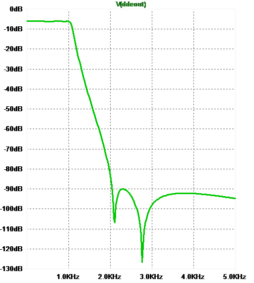
Figure 4: Frequency response of figure 3’s frequency-scaled filter.
What do we think of these component values? Calculating out those expressions, capacitors C``S and C``L have a value of 1/6283 F which is 159.1 uF. The series value of all the resistors “across the top” is only about 4.5 ohms. That doesn’t look easy to drive with standard op-amp circuitry; we’d need an audio power amplifier to push a signal through this. It’s not surprising, because we knew that our source and load capacitors were going to have an impedance of 1 ohm at 1 kHz (can you see why this is?).
So next, let’s also do some impedance scaling; we know how to do that. To make the circuit opamp-compatible, the resistor values are going to have to go up, and the capacitors will get lower in value to match. What about the D-elements? They are going to go down too, since their impedance is inversely proportional to the D value.
We’d get reasonable impedance values if we scaled by something like 10000, but actually, let’s use a value that makes the source and load capacitors a preferred value. 15915 does the trick because it takes those capacitors to 10 nF, which is pretty darned standard.

Figure 5: As figure 3, impedance scaled to make the caps 10nF.
The resulting network, this time with actual values, is shown in figure 5. Trust me, the frequency response plot is indistinguishable from figure 4. And, do you know what? We’re out of space again, and you still haven’t seen a single op-amp! Don’t worry, I promise I’ll rectify that omission soon, when we look at the classic circuit for implementing this filter actively. Meanwhile, happy de-inductoring!
[1] L. T. Bruton, “Frequency selectivity using positive impedance converter-type networks”. Proc. IEEE (Letters), vol. 56, pp 1378-1379, August 1968