Dualling Master: Swap Current and Voltage for Better Filter Design

We designed a passive lowpass ladder filter in “Filter Design using the Million Monkeys Method”. Well, I say “designed”, but really we just let Excel’s solver indulge in some cleverly-targeted component value adjustment. That way, we didn’t have to bother about optimization theory. We just made use of a general-purpose tool that’s widely available.

Using optimization to design circuits (some might call it organized guesswork – for some algorithms, that’s a pretty good description) isn’t a new insight. In the late 1960s, Ron Rohrer, teaching optimization at Berkeley, foresaw that the falling cost of numeric computation, and the rising complexity of electronic circuits, would eventually make circuit design-by-analysis cheaper and more effective than design-by-synthesis. All he needed was a way to analyze circuits effectively on a computer. Larry Nagel, the father of SPICE, was one of his students; the rest is history.

But back to our filters. In “Match Point: Why Maximum power means Minimum Sensitivity”, we discovered the handy insensitivity of the doubly-terminated ladder filter to component variations. This validates one of the choices made for the “Million Monkeys” design. But you’re all gasping to know how we’re actually going to use this well-behaved bunch of passive components to design a useful active filter. Some readers were a bit underwhelmed that the monkeys’ end product was just a bunch of interconnected Ls, Cs and Rs, producing a lowpass filter (albeit nice and sharp), cutting off at 0.159 Hz and having a very low input impedance. What use is that? After all, no-one uses passive filters down at this frequency, with inductors and capacitors that are both electrically and physically huge.

Now, I’ve got nothing against inductors (see “Fainting in Coils”). But there’s no doubt that active filters are way more popular and practical, at least in the sub-MHz region. No, these networks are not for use as actual filters. We use them as filter “prototypes”, seeds from which many useful inductorless filters can be grown, sharing many of the ladders’ attractive properties. The resulting filters are more manufacturable than the type of active filter in which first- and second-order filter sections are cascaded. So, how do we get started?

“It’s obvious”, the more vociferous audience members will say. “Just substitute the inductors with active circuits that have the same behavior as inductors”. In other words, you’re saying, find some snazzy combo of Rs, Cs and active devices that can masquerade as an inductor in our filter circuit. Now, I must play the “not enough space here” card and just declaim that this is a hard thing to do if the inductors don’t have one terminal connected to ground, based on filter design experience accumulated by many people over many decades. Imperfections in the inductance simulation blocks always cause some parasitic defects in the floating inductance created. One problem is that common-mode effects, particularly parasitic capacitance to the supply rails and other PCB traces, make it impossible to create a circuit that truly models a floating two-terminal component whose properties are independent of the potential of either terminal to ground. Sometimes the additional parasitic components to ground dominate the network behaviour and completely wreck the filter response. There can be circuit stability issues to contend with, as well; synthesized inductors may not always be stable under some loading conditions.

It turns out that we can make a good simulated grounded inductor; one day we’ll see how to make that and where it is useful. But first, we need to get another technique under our belts to move forward with our plans for the great Active Filters that I keep promising we’ll make.

To do this, I first need to take you back, back, back to “Simulate Circuits in a Spreadsheet with some Ladderal Thinking” and our analysis of ladder networks using a spreadsheet. To arrive at a value for the ladder’s attenuation, we carried out an iterative calculation down the ladder, using the following recurrence relations:

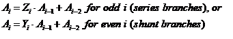
But, hang on a minute, these expressions have the same form. This implies that we should be able to make a network in which we interchange the role of impedances Z and admittances Y while keeping the values the same. That attenuation calculation algorithm will give the same result, as long as we start it off appropriately.

Any network can be defined by a set of equations relating node voltages and branch currents (a node is a point where components connect, and a branch is a connection between nodes). Have a look at figure 1:

Figure 1: an impedance Z forming a branch between nodes A and B.

Imagine if you will, ladies and gentlemen, another network in which current takes the place of voltage in these equations, and vice versa. In other words, for every branch AB in the original network for which we can write down

we can define a branch A`B` in the new network such that:

What we’ve done is to define the dual form of our original circuit. This circuit has nodes where the original had branches, and vice versa. Between any two ports (places where the network connects to the outside world), the new network has an impedance function that’s the reciprocal of the impedance of the original circuit (dual networks are also known as reciprocal networks). So, how do we construct this new network?

For a ladder, there’s an easy visualization of the transformation. Look at the uppermost section of figure 2, showing an impedance-led ladder network:

Figure 2: steps in forming the dual network of a ladder.

Imagine rotating each impedance or admittance through 90 degrees, and then reconnecting the branches in a new way shown by the green lines (center section of the figure). The resulting admittance-led ladder is redrawn in the bottom section. What were once impedances are now admittances with the same numeric value, and vice versa.

Our “Million Monkeys” example and its dual are shown in figure 3, including the source and load resistances. It’s important to note that this changes the topology; you are not just exchanging component types. The parallel combination of an L and a C is converted to a series combination of a C and an L – because impedances add in series, whereas admittances add in parallel. If you think about it, it should be clear that applying the same process a second time gets you back to the original network.

Figure 3: the “Million Monkeys” lowpass (on the left) and its dual (on the right).

Interpreting and using this network takes a little care. We have swapped the roles of voltage and current. This means that where, in the initial circuit, we applied an input voltage and inspected the output voltage, now we apply an input current and inspect the output current. If we have resistive source and load terminations, we can easily turn them back into voltage-mode connections, using Ohm’s law on the load R`L, and the Thevenin equivalent form of I1 in parallel with R`S for the source termination (hence the value of the current source I1).

These two networks are defined by the same equations and have identical sensitivity properties. In other words, the form on the right of figure 3 is just as robust against component variations as the original form on the left. The frequency responses are identical, so I don’t even need to plot them again.

We’ll need to pay attention if the termination resistor values weren’t unity to start with. If you look at the filter on the left side of figure 4 – already seen in “Match Point” – you’ll see that the load resistance RL for this singly-terminated filter is set to a gigaOhm, essentially infinite. This will translate into an essentially zero load impedance of a nanoOhm when we create the dual of this circuit. The current in this short-circuit load matches the voltage output of the original filter, but it’s clearly not much use if you want an output voltage from the filter. However, since the role of source and load can be interchanged (no room for the proof here!), we can run the network backwards to get a filter that can operate with zero source impedance and unit load impedance – see the right hand side of figure 4. It still has exactly the same, much poorer, sensitivity of the single-terminated filter (compared to a maximum-power matched doubly-terminated filter), but in a later column we’ll see that we nevertheless still sometimes find this configuration valuable.

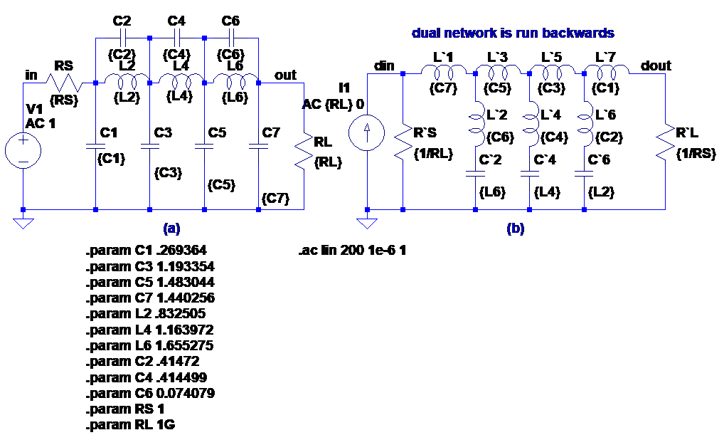
Figure 4: a single-terminated filter (note large RL), and its dual, driven backwards.

But hang on, you may say. The dual-form circuits clearly have at least twice as many inductors as the original circuit. You might think that this is a rather retrograde step, if our goal is to eliminate inductors! But we’re about to do something ever so beautiful in the next column, and all will become abundantly clear. How exciting – a cliffhanger ending. Meanwhile, happy dualling!