
When off-the-shelf won’t do: the step-by-step birth of a custom digital filter, Part 1
(Lightly edited from my old Planet Analog blog posts)

Some time back, I had to dig out some ancient filter design tools. I needed a special-purpose digital decimation filter for a “quite high quality” audio communication system. Of course, I was trying to cram this onto one of my then employer’s Programmable Systems on Chip (you know the acronym…).
I wrote an internal report on the design process, just in case anyone from the far future would be interested. I’ve split it into several Substack posts for all you filter fans out there. This is quite a complicated filter with several design constraints. Well, I thought it was; some of you MATLAB jocks out there might be able to do it in ten seconds while asleep these days. Whatever. I still think that occasionally designing something ‘longhand’ is a good way of highlighting constraints and how they affect the design process.
It’s designed as an analog lowpass filter and is transformed into the digital domain as late in the process as possible. The final filter is a 10th order filter; each of the two required signal channels will be implemented as a cascade of five Direct Form biquad sections on the hardware filter engine in that certain embedded processor,
step 1: choose passband and stopband frequencies
Passband choice was pretty simple, if only because people tend to give you a funny look if you defy audio convention in such matters. So, stuck as I was with an output (decimated) sample rate of 44.1 ksps, I went straight for a 20 kHz passband edge frequency, with a magnitude ripple of 0.1 dB peak-to-peak in the passband. Nothing too surprising there.
The system whose output this filter processes does some unconventional internal modulation and it throws up a full-scale modulated sideband pair centered around the input sampling frequency of 352.8 ksps. They get aliased back down to the baseband upon decimation. The frequencies ‘go back to where they came from’, so this isn’t audibly harmful. But the passband frequency response will be altered by these components adding to or subtracting from the existing baseband signal, so we’ll need the stopband attenuation of the filter to be high enough that the overall response doesn’t deviate too much.
To achieve this, I defined the primary stopband to extend 20 kHz either side of 44.1 kHz, i.e. from 24.1 kHz to 64.1 kHz. A stopband attenuation of at least 46 dB between these frequencies will ensure that the extra passband ripple caused by the aliased components is less than ±0.086 dB. As for the inherent passband ripple, I went for ±0.05 dB, giving us a worst possible passband ripple of ±0.136 dB, which is acceptable for this particular moderate quality system.
Why only define the stopband over a finite range of frequencies? Because sometimes you can get more attenuation where you need it, if you don’t ask for attenuation at frequencies where you don’t actually need it. As it happens, in this particular case forcing the attenuation over this range of frequencies also ensured that it was at least that good at higher frequencies. It doesn’t always work out that way.
The filter is driven from a source with an out-of-band noise floor that’s rising at +18 dB per octave (it’s actually the output of a processed and partially-filtered delta-sigma modulator). To stop this from becoming an issue, we’ll need a stopband rejection slope of at least -18 dB per octave in the frequency range where the noise is rising like this. This is another way of saying this is that there are (at least) three transmission zeroes at infinity. That means that we shouldn’t use ‘catalog’ elliptic filters, which have a maximum final high frequency stopband slope of -12 dB per octave in even-order form.
One more thing: because this analog filter will eventually be transformed into the digital domain using the bilinear transform, we’ll need to ‘prewarp’ our design frequencies. This is done to ensure that the final passband and stopband frequencies are in the desired place after the transform. The bilinear transform ‘warps’ the frequency axis, with the digital filter’s features always ending up at a somewhat lower frequency compared to their starting point in the analogue domain. Taking this into account means that the design passband edge for the initial analogue filter should be at 20.21417 kHz. OK, that’s only a 1% difference. The amount by which you need to shift the frequency can really shoot up if your sample rate isn’t a high multiple of the frequency point being warped, though. The warped stopband points are 24.47692 kHz and 72.10644 kHz; that upper one has shifted up by a significant 12.5%.
step 2: generate an s-domain polynomial for the basic lowpass response
The solution used here to define both an arbitrary stopband and a specific upper stopband slope is to use a ‘zero placer’ program of the type that delivers an equiripple (i.e. flat to within a maximum ripple value) passband with a user-defined count of finite and infinite poles. I dug out some of my ancient self-penned filter design tools to do this (containing code that dates back to the early 80s, informed by classic filter design texts dating back to the 60s).
This trusty old code confirmed that the filter requirements were indeed achievable with a 7th order prototype lowpass function with two finite stopband zeroes and three zeroes at infinity (there’s my -18 dB per octave), with at least 47.5 dB of stopband rejection.
Figures 1 and 2 give a peek at the responses of the filter so far. Figure 1 extends up to 352.8 kHz simply because next time I want to overlay the response of the digital filter which we end up with, and I’ll use that same scaling.
Figure 2 shows a classic equiripple passband, and also (the fainter dotted line) the group delay (it’s the derivative of the phase shift with frequency). This takes us neatly to the next step…
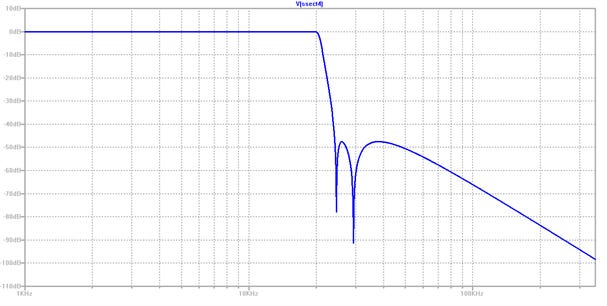
Figure 1: Passband and stopband magnitude, up to 352.8 kHz, log scale
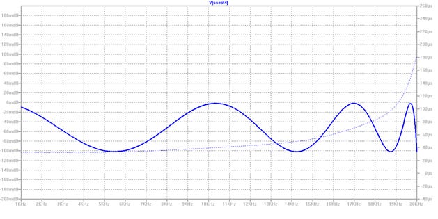
Figure 2: Passband magnitude and group delay, up to 20 kHz
step 3: phase-equalize for better behavior on audio signals
Minimum-phase filters with equiripple passbands that turn over rapidly to a fast-falling stopband inevitably have pretty poor phase linearity in the passband (figure 2 shows the rising group delay from the filter so far). While studies into the audibility of such phase deviations are inconclusive, they are generally considered to be unacceptable in a modern audio system intended for full bandwidth reproduction. Since the other methods used for creating decimation filters in audio converters are either approximately or exactly linear phase, it’s important not to be at a marketing disadvantage by allowing bad phase non-linearity here. Perhaps my audio heritage makes me want to over-engineer here. But I’m a filter guy, so I want to do the best job I can, given implementation constraints, for both audio fun and filter fun.
A modest amount of phase equalization is therefore applied to the filter. A good target is to get the phase response to fit a straight line (through zero) to within a degree or two over most of the (audible) audio band. I ended up performing the phase equalization using response data from DC up to 18.4 kHz, which I think is adequate here. The analogue anti-aliasing and anti-imaging filters for the first generation of digital mixing desks in the 80s were phase-equalized only up to about 16 kHz and they sounded fine (I know, ‘cos I designed them).
I used more very old software of my own design (hands up, anyone who remembers the BBC Micro… that’s what I used in the early 80s when I started writing this sort of stuff) to do the phase equalization. My guess was that a 3rd order phase equalizer would get somewhere close. This is neat because then the total order of the filter is 10, meaning five 2nd order biquads (and I know we can do two such 10th order filters at the desired input sample rate on the filter engine in the target embedded device – something no MCU core could do at the time, by the way…). The first-order sections from the 7th order filter and from the 3rd order equalizer are combined into one biquad for ease of coding (the slight noise floor impairment this can potentially cause when Direct Form biquads are used is not an issue in this particular system).
The bilinear transform (which turns our analog filter functions into digital ones) introduces a little grief for us at the phase equalization stage too. An analog filter with a phase shift that’s a linear function of ‘analog frequency’ will transform to a digital filter whose phase shift is not a linear function of actual frequency, but is ‘bent’ by the warping effect.
One solution to this (the one that best fits my own old software!) is to adjust the equalizer coefficients so that the response is a best fit not to a straight line but to a curve that becomes a straight line after warping. In my software this was easily achieved by prewarping the frequency values of the phase response data set used in the optimization (without ‘telling’ the linear regression calculation). All that’s needed is a knowledge of the sample rate you’re going to use. In passing, it’s interesting to note that the ‘bend’ required is in the opposite direction to the way that the unequalized filter’s phase response is already bending. In other words, the need to allow for the bilinear transform makes the phase equalization more demanding.
Suitably modified, the software gave the parameters for a suitable 3rd order phase equalizer (an allpass filter with a flat magnitude response but a phase response whose frequency variation linearizes the phase response of the starting filter). However, the software calculates parameters for an analog equalizer, so we also need to prewarp the pole and zero frequencies so that when we perform the bilinear s-to-z transform on the equalizer, the parameters end up where we want them. Confusing? No wonder they call this process ‘warping’!
There are a few more steps to take in the analog domain before we go through the s-to-z looking-glass. Next time I’ll look at how we ensure that we combine and order the filter poles and zeroes so that we get the best possible signal-handling performance. It’s easy to assume that ‘digital is perfect’ and that you don’t have to worry about component performance like you do in the analogue world. That’s not true – check out here and here for some insight into the noisiness of digital filters. And check back soon to pick up the trail and see the final results!