Countdown to s-to-z…

Extra pop-quiz points for getting the pun

The technique in this piece will help us move on from both “an Excelent Fit, Sir!” and “When off the shelf won’t do”. In the first of those, we used Excel’s ‘solver’ functionality to bend a filter transfer function to our will. Or, rather, our customer’s will, since s/he is much more important than we ever are.

Now, our customer likely doesn’t want to buy big, expensive, high-quality capacitors to build an active filter with the response we derived. So, having established the principle of optimizing in the analog domain, let’s look at whether need to make any changes in order to use it to create a digital filter for our preferred embedded or digital processing platform.

Well, the first thing to do is to choose a sample rate. The noise bandwidth of our system will be dominated by this equalizing filter, whose response falls at 6 dB per octave above about 30 Hz. If we set the intrinsic sample rate too high, we’ll use power unnecessarily and may have to watch for arithmetic issues in the subsequent digital filter (see “Which filters are Noisier”). If we set the sample rate too low, then the inherent response of the ADC’s decimation and/or input filters may have to be accounted for (see “Now Fix those drooping ADC and DAC Responses”).

Well, we need not worry; if we pick a sample rate of 1 ksps, these issues should be completely negligible. Another more advanced digital filter design issue called ‘frequency warping’ can also be completely ignored (this is going to come up in the next piece in the “When off the shelf won’t do” sequence).

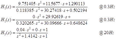
Even-order harmonics of the AC line frequency will cause a modulation of the incident light level (dang! I’ve given the game away, yes, it is a PIR sensor). We can address this potential interferer with some extra filtering. So, just because we can, I’ve put in another lowpass filter section designed to be flat up to 10 Hz (our equalization limit), and I’ve also sneakily dropped in a notch (technically a ‘zero) at 100 Hz, which is where most of the trouble is going to be, in Europe or China anyway. I used a ‘Butterworth’-aligned section, which has a dissipation factor of sqrt(2); positioned the ‑3 dB point out of the way at 20 Hz, and instead of leaving the a2 coefficient at 0, I made it equal to 1/25, which gives a zero at sqrt(25) times the 20 Hz normalization frequency, i.e. 100 Hz. After a final ‘solve’, Excel gives:

We can’t put it off any longer; let’s make that move from the s-domain to the z-domain. A spreadsheet is certainly a nice warm place for the s-to-z transform to hide. Here we’re going to use the most common way of crossing between those domains, usually referred to as the bilinear transform. To save your eyes from going all woogly I’ve put the derivation we need in an appendix at the end of the piece.

Using this method gives the coefficients of powers of z in H(z), which translate more or less directly to the actual multiplication factors used in the digital filter sections, depending on the particular topology you use. What now remains in the last few hundred words is to work out the transfer function, and then run it through a simulator to show that it does indeed do what it “says on the tin”.

So that you can check your own work, here are the coefficients in standard equation form that I ended up with for the three filter sections in table 1 (your optimizations may be slightly different):

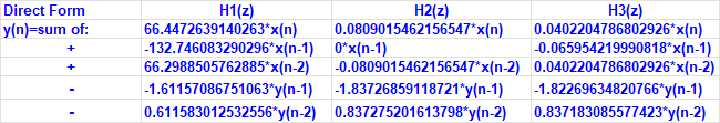
Table 1: the three filter sections in equation form (note signs for the Direct Form code)

I’ll wheel out trusty LTspice to analyze the filter. The block I use is a z-domain analog Direct Form biquad model that is built using transmission lines as delay elements. It runs cleanly and quickly in both time and frequency domains. I embed the whole circuit in ASCII schematic form in another sheet in the Excel file; it picks up the design values directly from the s-to-z transform sheet. Just paste the worksheet back to a text file with .asc extension and it opens straight up with LTspice (figure 1):

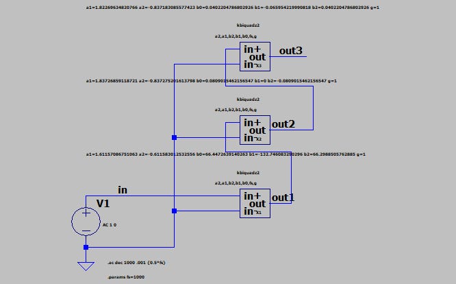
Figure 1: simple analysis of the digital biquad.

Finally the suspense is over: here’s the response of the final filter (figure 2). The notch at 100 Hz can clearly be seen, as can the fall to another notch at 500 Hz – half the sample rate – which is characteristic of a digital filter designed with the bilinear transform method:

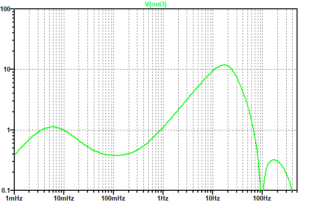
Figure 2: the final realized response of the digital “An Excelent fit, Sir!” filter.

This is just a whistle-stop tour through this design approach. I’ll talk about a more elaborate filter using this design flow leading from analog to digital shortly. But meanwhile, do you… sense… that this approach might help you with your sensor-enabled hardware?

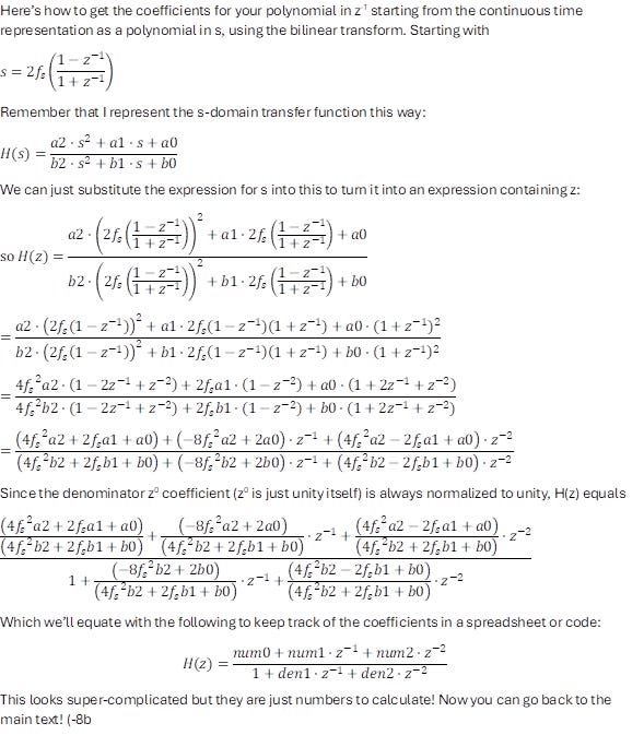
Appendix: the calculation of z-domain coefficients from s-domain coefficients

Note: this is a single image; the integration between MS Word equation stuff and Substack is a bit sucky, on perhaps I’m just not very good at the formatting…